Transformations

상위: Spark

요약

Spark 연산은 Transformation과 Action으로 구분됩니다. Transformation은 새로운 RDD를 생성하는 설계도이고, Action은 실제 실행 버튼입니다. Transformation은 Narrow와 Wide로 나뉘며, Lazy Evaluation으로 최적화됩니다.

Transformation vs Action

Spark 연산은 크게 Transformation + Action으로 구별됨

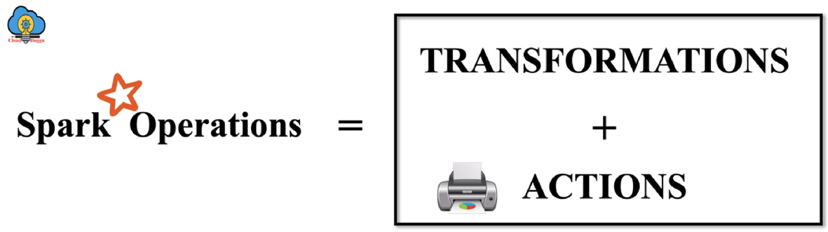
• Transformation: 설계도
• Action: 실행 버튼

Transformation

• immutable(불변)인 원본 데이터를 수정하지 않고, 하나의 RDD나 DataFrame을 새로운 RDD나 DataFrame으로 변형
• (input, output) 타입: (RDD, RDD), (DataFrame, DataFrame)
• 예: map(), filter(), flatMap(), select(), groupby(), orderby()
• Narrow, Wide Transformation 두 종류 존재

Action

• immutable(불변)인 입력에 대해 Side effect(부수 효과)를 포함하고, 아웃풋이 RDD 혹은 DataFrame이 아닌 연산
• 예:
  • count() → int
  • collect() → array
  • save() → void

Narrow Transformation

→ Stage가 나뉘지 않고 그대로 유지

• input: 1개의 파티션
• output: 1개의 파티션
• 파티션 간의 데이터 교환이 발생하지 않음

→ 각 파티션은 자기 안에서만 연산을 처리

예시: filter(), map(), coalesce() (Partition 수 줄임)

Narrow Transformation 특징

• 빠른 성능: 네트워크 통신 불필요
• 파이프라이닝 가능: 여러 Narrow Transformation을 하나의 Stage에서 연속 실행
• 장애 복구 용이: 해당 파티션만 재계산

Narrow Transformation 예시

# filter: 각 파티션 독립적으로 필터링
rdd = sc.parallelize([1, 2, 3, 4, 5, 6], 3)
filtered = rdd.filter(lambda x: x % 2 == 0)
# Partition 0: [1, 2] → [2]
# Partition 1: [3, 4] → [4]
# Partition 2: [5, 6] → [6]

# map: 각 요소 독립적으로 변환
mapped = rdd.map(lambda x: x * 2)
# Partition 0: [1, 2] → [2, 4]
# Partition 1: [3, 4] → [6, 8]
# Partition 2: [5, 6] → [10, 12]

Wide Transformation

→ Stage 분리

→ Stage 수 = Shuffle 일어나는 수 + 1

• 연산 시 파티션끼리 데이터 교환 발생
• 예: groupby(), orderby(), sortByKey(), reduceByKey()
• 단, join의 경우 RDD/DataFrame의 파티셔닝 방식에 따라 narrow일 수도, wide일 수도 있음

Wide Transformation 특징

• Shuffle 발생: 네트워크를 통한 데이터 재분배
• 성능 비용 높음: 디스크 I/O, 네트워크 I/O 발생
• 새로운 Stage 생성: Shuffle 경계에서 Stage 분리
• 메모리 사용 증가: 중간 데이터 버퍼링

Wide Transformation 예시

# groupByKey: 같은 키를 가진 데이터를 한 파티션으로 모음
rdd = sc.parallelize([("A", 1), ("B", 2), ("A", 3), ("B", 4)], 2)
grouped = rdd.groupByKey()
# Shuffle 발생: 모든 "A"는 하나의 파티션으로, 모든 "B"는 다른 파티션으로

# reduceByKey: 키별로 집계 (로컬 + 글로벌)
reduced = rdd.reduceByKey(lambda a, b: a + b)
# 로컬 reduce 후 Shuffle, 다시 reduce

Narrow vs Wide 판단

Lazy Evaluation

• 모든 transformation은 즉시 계산되지 않고 **계보(lineage)**라 불리는 형태로 기록됨
• transformation이 실제 계산되는 시점은 action이 실행되는 시점
• action이 실행될 때, 그 전까지 기록된 모든 transformation들의 지연 연산이 수행됨

Lazy Evaluation 장점

1. 쿼리 최적화

• 스파크가 연산 쿼리를 분석하고, 어디를 최적화할지 파악하여 실행 계획 최적화 가능
• (cf. eager evaluation은 즉시 연산이 수행되므로 최적화 여지가 없음)

예시:

# Spark는 다음 연산을 한 번에 분석
rdd = sc.textFile("data.txt")
result = rdd.filter(lambda x: "ERROR" in x) \
            .filter(lambda x: "2024" in x) \
            .count()

# 최적화: 두 filter를 하나로 합침
# optimized: filter(lambda x: "ERROR" in x and "2024" in x)

2. 데이터 내구성 제공

• 장애에 대한 데이터 내구성 제공
• 장애 발생 시, 스파크는 기록된 lineage를 재실행하는 것만으로 원래 상태를 재생성할 수 있음

→ cf. Savepoint, checkpoint

3. 불필요한 연산 방지

# 만약 eager evaluation이라면 모든 map이 실행됨
rdd = sc.parallelize([1, 2, 3, 4, 5])
mapped = rdd.map(lambda x: x * 2)  # eager면 여기서 실행
result = mapped.take(2)  # lazy: 2개만 처리하면 됨을 알고 최적화

# Spark는 2개만 처리해도 된다는 것을 알고 있음

Transformation & Action의 실행 계획

1. Transformation 단계

rdd1 = sc.textFile("data.txt")           # Lineage 기록
rdd2 = rdd1.map(lambda x: x.upper())     # Lineage 기록
rdd3 = rdd2.filter(lambda x: "SPARK" in x)  # Lineage 기록
# 아직 실행 안 됨!

2. Action 단계

result = rdd3.count()  # 이제 모든 Transformation 실행!

실행 순서:

1. DAG Scheduler가 Lineage 분석
2. Stage 분리 (Shuffle 기준)
3. Task 생성 (파티션 기준)
4. Executor에 Task 전달
5. 결과 수집

Stage와 Transformation의 관계

rdd = sc.textFile("data.txt")
# Stage 0 시작
rdd2 = rdd.map(lambda x: x.split(","))      # Narrow → Stage 0
rdd3 = rdd2.filter(lambda x: len(x) > 3)    # Narrow → Stage 0
# Stage 0 끝, Stage 1 시작 (Shuffle 발생)
rdd4 = rdd3.groupByKey()                     # Wide → Stage 1
rdd5 = rdd4.mapValues(lambda x: sum(x))     # Narrow → Stage 1
result = rdd5.collect()                      # Action 실행

# 총 2개 Stage (1번의 Shuffle)

최적화 팁

1. Wide Transformation 최소화

# Bad: 여러 번 Shuffle
rdd.groupByKey().mapValues(sum)

# Good: 한 번에 집계
rdd.reduceByKey(lambda a, b: a + b)

2. Narrow Transformation 활용

# Bad: 데이터 먼저 가져온 후 필터링
rdd.collect()
filtered = [x for x in rdd if x > 10]

# Good: 필터링 후 가져오기
rdd.filter(lambda x: x > 10).collect()

3. Partition 관리

# Bad: 불필요한 repartition
rdd.repartition(100).filter(...)

# Good: 필요한 만큼만
rdd.filter(...).coalesce(10)

4. 캐싱 활용

반복 사용 시 cache()로 중간 결과 재사용 → 상세는 RDD Actions.